Org to Reveal.js
(Reveal.js Cheatsheet)
Tae Eun Kim, Ph.D.
Reveal.js and Org-Reveal
Reveal.js is a tool for creating good-looking HTML presentations, authored by Hakim El Hattab.
For an example of a reveal.js presentation, see here.
Org-Reveal exports your Org documents to reveal.js presentations.
With Org-reveal, you can create beautiful presentations with 3D effects from simple but powerful Org contents.
Codes
You can also install the latest developing version of org-reveal directly from GitHub.
Please download the latest Org-reveal package from the Org-reveal GitHub page. Or clone the GitHub repository:
git clone https://github.com/yjwen/org-reveal.gitCopy
ox-reveal.elto one of your Emacs'sload-path, and add the following statement to your.emacsfile.(require 'ox-reveal)Note: It is suggested to use the Org-mode git repository in pair with the GitHub org-reveal. Please get the Org-mode git repository by:
$ git clone https://code.orgmode.org/bzg/org-modeFollow the online instruction for building and installing Org-mode.
MATLAB code
 function x = fpi(g, x0, n)
 % FPI x = fpi(g, x0, n)
 % Computes approximate solution of g(x)=x
 % Input:
 %   g    function handle
 %   x0   initial guess
 %   n    number of iteration steps
     x = x0;
     for k = 1:n
         x = g(x);
     end
 end

 f = @(x) x.^2 - 4*x + 3.5;
 g = @(x) x - f(x);
 fplot(g, [2 3], 'r');
 hold on
 plot([2 3], [2 3], 'k--')
 x = 2.1;
 y = g(x);
 for k = 1:5
     arrow([x y], [y y], 'b');
     x = y; y = g(x);
     arrow([x x], [x y], 'b');
 end
Images
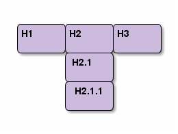
Assume we have a simple Org file as below:
* H1
* H2
** H2.1
*** H2.1.1
* H3
Images
If HLevel is 1, the default value, headings H2.1 and H2.1.1 will be mapped to vertical slides below the slides of heading H2.
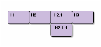
If HLevel is changed to 2, slides of heading H2.1 will be changed to the main horizontal queue, and slides of heading H2.1.1 will be a vertical slide below it.
More Images
- Array creation

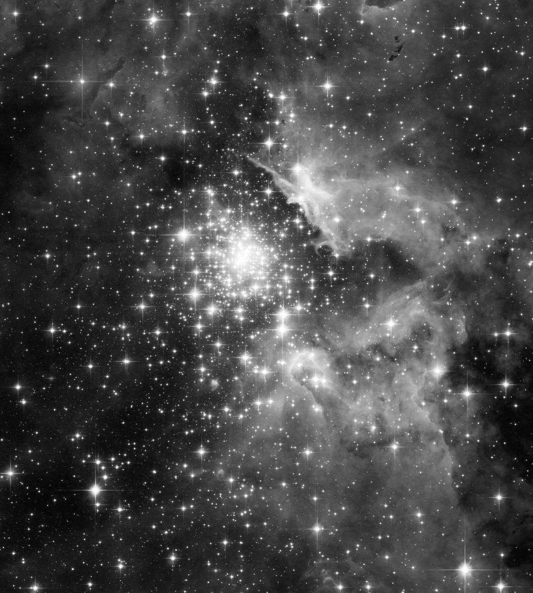
More Images
- Hubble
Lorenz Equation
The Lorenz system is \(\begin{aligned} \dot{x} & = \sigma(y-x) \\ \dot{y} & = \rho x - y - xz \\ \dot{z} & = -\beta z + xy \end{aligned}\)
More Maths
The rootfinding problem \(f(x) = x^3 + x - 1 = 0\) can be transformed to various fixed point problems:
- \(g_1(x) = x - f(x) = 1 - x^3\)
- \(g_2(x) = \sqrt[3]{1 - x}\)
- \(\ds g_3(x) = \frac{1+2x^3}{1+3x^2}\)
Note that all \(g_j(x) = x\) are equivalent to \(f(x)=0\). However, not all these find a fixed point of \(g\), that is, a root of \(f\) on the computer.
Exercise. Run fpi with \(g_j\) and \(x_0 = 0.5\). Which fixed point iterations converge?
Two Columns: Pro/Con of emacs-reveal
Pros
- Free/libre open source software
- Device-independent presentations
- Also mobile and offline
- Generated from simple text format
- Easy to learn
- Collaboration with diff/merge/git
- Separation of layout and content
Cons
- No WYSIWYG
- (Need to learn something new)
Environments (boxes)
Problem: Fitting Functions to Data
Given data points \(\{ (x_i, y_i) \mid i \in \NN[1,m]\}\), pick a form for the ``fitting'' function \(f(x)\) and minimize its total error in representing the data.
- With real-world data, interpolation is often not the best method.
- Instead of finding functions lying exactly on given data points, we look for ones which are ``close'' to them.
- In the most general terms, the fitting function takes the form \[ f(x) = c_1 f_1(x) + \cdots + c_n f_n(x), \] where \(f_1, \ldots, f_n\) are known functions while \(c_1, \ldots, c_n\) are to be determined.
Linear Least Squares Approximation
Tables
Below are 5-year averages of the worldwide temperature anomaly as compared to the 1951-1980 average (source: NASA).
| Year | Anomaly (\(^{\circ}C\)) |
|---|---|
| 1955 | -0.0480 |
| 1960 | -0.0180 |
| 1965 | -0.0360 |
| 1970 | -0.0120 |
| 1975 | -0.0040 |
| 1980 | 0.1180 |
| 1985 | 0.2100 |
| 1990 | 0.3320 |
| 1995 | 0.3340 |
| 2000 | 0.4560 |
Discussions
In this discussion: \vs
- use a polynomial fitting function \(p(x) = c_1 + c_2 x + \cdots + c_n x^{n-1}\) with \(n < m\);
- minimize the 2-norm of the error \(r_i = y_i - p(x_i)\): \[ \Norm{\br}{2} = \sqrt{\sum_{i=1}^m r_i^2} = \sqrt{\sum_{i=1}^{m} \left( y_i - p(x_i) \right)^2}. \]
\vs Since the fitting function is linear in unknown coefficients and the 2-norm is minimized, this method of approximation is called the linear least squares (LLS) approximation.